Towards a Deeper Understanding of SGS Models in Large Eddy Simulation

I wrote about SGS models for LES about eight years ago. In that post, ILES was advocated for wall-resolved LES with dissipative high-order methods such as the discontinuous Galerkin, spectral difference, and flux reconstruction (FR) methods. Many groups, including us, showed that adding SGS models produced worse results than ILES compared to DNS results. 

We did find an outlier earlier this year. An SGS model improved the results of LES of the turbulent channel flow with a 6th-order (P5) FR scheme. A further investigation leads to a deeper understanding of SGS models in LES. Here are the main findings:

• The SGS stress is a 2nd-order term with respect to the filter size or mesh size. This means any schemes higher than 2nd order do not have enough dissipation to damp the sub-grid scales, resulting in energy pileups near the cut-off wave number as shown in Figure 1.      

Figure 1. Energy spectra for ILES of Burgers turbulence with different P orders

• The energy pileups for P2, P3 and P4 schemes appear to improve the prediction of the wall skin friction compared to the DNS results. In other words, the unphysical energy addition due to unresolved scales appears to compensate for the energy loss (relative to DNS) due to the LES filtering, resulting in a better agreement with DNS data. Any damping of these pileups pushes the results further away from the DNS data.  
  
  
• On the other hand, the P5 scheme over-compensated for the energy loss, and the addition of an SGS model can achieve a better agreement with DNS data. This also means that very coarse meshes can be used with the P5 scheme to achieve DNS-like results with a properly calibrated SGS model.  

In summary, use ILES with any schemes lower than 6th order (P2-P4), but use an SGS model with 6th or higher order schemes (P > 4). The findings will be presented in SciTech 2026 at Orlando. I will also play pickleball in Orlando Racket Sports. If you are interested in learning or playing pickleball in Orlando, do let me know.

 A Perfect Celebration

On December 5-7, 2024, a symposium, Emerging Trends in Computational Fluid Dynamics: Towards Industrial Applications, was successfully held at Stanford University to celebrate the 90th birthday of CFD legend, Professor Antony Jameson. I am very grateful to Antony for giving Professor Chongam Kim and myself an opportunity to celebrate our 60th birthday in conjunction with his. Thus, the symposium is also called the Jameson-Kim-Wang (JKW) symposium.

An organizing committee led by Professor Siva Nadarajah (McGill University) and composed of Professors Chunlei Liang (Clarkson University), Meilin Yu (UMBC), and Hojun You (Sejong University) did a fantastic job in organizing a flawless symposium. The list of speakers includes the who's who and rising stars in CFD. A special shoutout goes to Professor Juan Alonso and the sponsors for their support of the Symposium.  A photo of the attendees is shown in Figure 1. Some good-looking posters from the sponsors are shown in Figure 2.

Figure 1. Attendees of the JKW Symposium

Figure 2. Posters from some of the sponsors

Antony's many pioneering contributions to CFD have been well documented in the literature. His various CFD and design optimization codes have shaped the design of commercial aircraft for many decades. Several aircraft manufacturers told stories about Antony's impact. We look forward to the release of the Symposium videos next year. 

Next, I'd like to touch upon my personal connection to Antony. I first heard of his name and his work in China from my graduate advisor, Academician Zhang Hanxin. I still recall reading his paper on the successes and challenges in computational aerodynamics. I believe I first met Antony at an AIAA conference when he came to my talk on conservative Chimera. I did not get an opportunity to introduce myself. Our 2nd meeting took place in China during an Asian CFD conference in 2000 where both of us were invited speakers. We sat at the same table with Charlotte (Mrs. Jameson) in a banquet. This time I was able to properly introduce myself. 

Soon after that, we started collaborating on high-order methods, from spectral difference to flux reconstruction. I visited Antony's lab and co-organized his 70th birthday celebration at Stanford in late 2004. During a visit to his home, Antony shared his fascination on the aerodynamics of hummingbirds. I still recall receiving his phone call about proving the stability of the SD method with Gauss points as the flux points on a Saturday when I was at my son's soccer game! 

The Symposium also gave me an opportunity to see many of my former students, some of whom I have not seen for more than two decades: Yanbing, Khyati, Prasad, Chunlei, Varun, Takanori, Meilin, Lei, Cheng, Feilin, Eduardo and Justin. It is very gratifying to hear their stories after so many years.

Figure 3. Group photo after a great dinner

The Symposium concluded with an amazing banquet. My friend and collaborator, H.T. Huynh, did a hilarious roast of me and I cannot stop laughing the whole time. H.T. has the talent of a standup comedian. Everything went smoothly and we had a perfect symposium!

Note on RANS, Hybrid RANS/LES, WRLES, WMLES and SGS Models

 In the computation of turbulent flow, there are three main approaches: Reynolds averaged Navier-Stokes (RANS), large eddy simulation (LES), and direct numerical simulation (DNS). LES and DNS belong to the scale-resolving methods, in which some turbulent scales (or eddies) are resolved rather than modeled. In contrast to LES, all turbulent scales are modeled in RANS.

Another scale-resolving method is the hybrid RANS/LES approach, in which the boundary layer is computed with a RANS approach while some turbulent scales outside the boundary layer are resolved, as shown in Figure 1. In this figure, the red arrows denote resolved turbulent eddies and their relative size. 

Depending on whether near-wall eddies are resolved or modeled, LES can be further divided into two types: wall-resolved LES (WRLES) and wall-modeled LES (WMLES). To resolve the near-wall eddies, the mesh needs to have enough resolution in both the wall-normal (y+ ~ 1) and wall-parallel directions (x+ and z+ ~ 10-50) in terms of the wall viscous scale as shown in Figure 1. For high-Reyolds number flows, the cost of resolving these near-wall eddies can be prohibitively high because of their small size. 

In WMLES, the eddies in the outer part of the boundary layer are resolved while the near-wall eddies are modeled as shown in Figure 1. The near-wall mesh size in both the wall-normal and wall-parallel directions is on the order of a fraction of the boundary layer thickness. Wall-model data in the form of velocity, density, and viscosity are obtained from the eddy-resolved region of the boundary layer and used to compute the wall shear stress. The shear stress is then used as a boundary condition to update the flow variables.    

Figure 1. An illustration of RANS, hybrid RANS/LES, WRLES, and WMLES approaches

I discussed the role of sub-grid scale (SGS) models for WRLES in an earlier blog post in 2017. For adaptive high-order methods such as the discontinuous Galerkin (DG), spectral difference (SD), and flux reconstruction/correction procedure via reconstruction (FR/CPR) methods, the best results are obtained without any explicit SGS models (called implicit LES or ILES) because of the embedded numerical dissipation. With enough mesh resolution, the physical and numerical dissipations appear sufficient to stabilize WRLES.

In WMLES, the near-wall turbulent scales are severely under-resolved. As a result, ILES is usually not stable without other stabilizing techniques such as filtering, limiting et al. We recently experimented with explicit SGS models such as the Smagorinsky, WALE, and Vreman models for WMLES. Through comparison with channel flow DNS data, the Vreman model was found to achieve the most accurate and consistent results. 

In summary, we advocate ILES for WRLES and the Vreman model for WMLES with adaptive high-order methods such as DG, SD, and FR/CPR. 

     

  

Is High-Order Wall-Modeled Large Eddy Simulation Ready for Prime Time?

During the past summer, AIAA successfully organized the 4th High Lift Prediction Workshop (HLPW-4) concurrently with the 3rd Geometry and Mesh Generation Workshop (GMGW-3), and the results are documented on a NASA website. For the first time in the workshop's history, scale-resolving approaches have been included in addition to the Reynolds Averaged Navier-Stokes (RANS) approach. Such approaches were covered by three Technology Focus Groups (TFGs): High Order Discretization, Hybrid RANS/LES, Wall-Modeled LES (WMLES) and Lattice-Boltzmann.

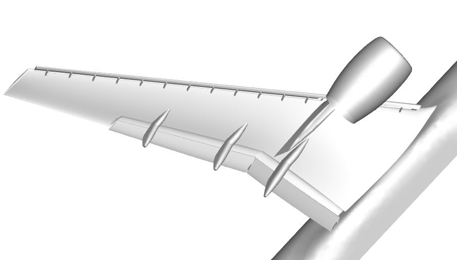
The benchmark problem is the well-known NASA high-lift Common Research Model (CRM-HL), which is shown in the following figure. It contains many difficult-to-mesh features such as narrow gaps and slat brackets. The Reynolds number based on the mean aerodynamic chord (MAC) is 5.49 million, which makes wall-resolved LES (WRLES) prohibitively expensive.

The geometry of the high lift Common Research Model

University of Kansas (KU) participated in two TFGs: High Order Discretization and WMLES. We learned a lot during the productive discussions in both TFGs. Our workshop results demonstrated the potential of high-order LES in reducing the number of degrees of freedom (DOFs) but also contained some inconsistency in the surface oil-flow prediction. After the workshop, we continued to refine the WMLES methodology. With the addition of an explicit subgrid-scale (SGS) model, the wall-adapting local eddy-viscosity (WALE) model, and the use of an isotropic tetrahedral mesh produced by the Barcelona Supercomputing Center, we obtained very good results in comparison to the experimental data. 

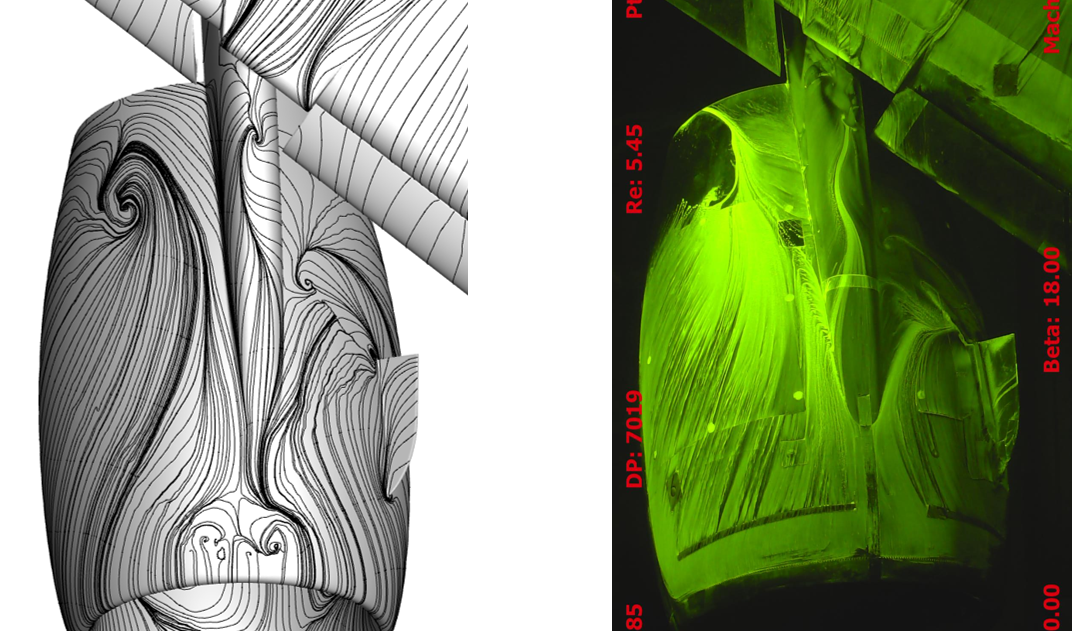
At the angle of attack of 19.57 degrees (free-air), the computed surface oil flows agree well with the experiment with a 4th-order method using a mesh of 2 million isotropic tetrahedral elements (for a total of 42 million DOFs/equation), as shown in the following figures. The pizza-slice-like separations and the critical points on the engine nacelle are captured well. Almost all computations produced a separation bubble on top of the nacelle, which was not observed in the experiment. This difference may be caused by a wire near the tip of the nacelle used to trip the flow in the experiment. The computed lift coefficient is within 2.5% of the experimental value. A movie is shown here.        

Comparison of surface oil flows between computation and experiment 

Comparison of surface oil flows between computation and experiment 

Here are some lessons we learned from this case. Besides the space and time discretization methods, the computational mesh and the SGS model strongly affect WMLES results. 

• Since we obtain wall model data from the 2nd element away from the wall, it is important that isotropic elements be used near solid walls to ensure that turbulent eddies are resolved well there. That's why we prefer tetrahedral elements for complex geometries since one can always generate isotropic elements. In other words, inviscid meshes are preferred for WMLES!
  
  
• For very under-resolved turbulent flow, the use of an explicit SGS model such as WALE produces more accurate and robust results than a shock-capturing limiter. It is quite difficult to determine the appropriate amount of limiting.  

The recent progress has been documented in an AIAA Journal paper, and an upcoming conference paper in SciTech 2023. The latest high-order results indicate that high-order LES can reduce the total DOFs by an order of magnitude compared to 2nd order methods. We believe it is ready for prime time for high-lift configurations, turbomachinery, and race car aerodynamics. You are welcome to try high-order WMLES by getting the flow solver from www.hocfd.com.   

   

A Benchmark for Scale Resolving Simulation with Curved Walls

Multiple international workshops on high-order CFD methods (e.g., 1, 2, 3, 4, 5) have demonstrated the advantage of high-order methods for scale-resolving simulation such as large eddy simulation (LES) and direct numerical simulation (DNS). The most popular benchmark from the workshops has been the Taylor-Green (TG) vortex case. I believe the following reasons contributed to its popularity:

• Simple geometry and boundary conditions;
• Simple and smooth initial condition;
  
• Effective indicator for resolution of disparate space/time scales in a turbulent flow.
  

Using this case, we are able to assess the relative efficiency of high-order schemes over a 2nd order one with the 3-stage SSP Runge-Kutta algorithm for time integration. The 3rd order FR/CPR scheme turns out to be 55 times faster than the 2nd order scheme to achieve a similar resolution. The results will be presented in the upcoming 2021 AIAA Aviation Forum.

Unfortunately the TG vortex case cannot assess turbulence-wall interactions. To overcome this deficiency, we recommend the well-known Taylor-Couette (TC) flow, as shown in Figure 1.

 

Figure 1. Schematic of the Taylor-Couette flow (r_i/r_o = 1/2)

The problem has a simple geometry and boundary conditions. The Reynolds number (Re) is based on the gap width and the inner wall velocity. When Re is low (~10), the problem has a steady laminar solution, which can be used to verify the order of accuracy for high-order mesh implementations. We choose Re = 4000, at which the flow is turbulent. In addition, we mimic the TG vortex by designing a smooth initial condition, and also employing enstrophy as the resolution indicator. Enstrophy is the integrated vorticity magnitude squared, which has been an excellent resolution indicator for the TG vortex. Through a p-refinement study, we are able to establish the DNS resolution. The DNS data can be used to evaluate the performance of LES methods and tools. 

 

Figure 2. Enstrophy histories in a p-refinement study

A movie showing the transition from a regular laminar flow to a turbulent one is posted here. One can clearly see vortex generation, stretching, tilting, breakdown in the transition process. Details of the benchmark problem has been published in Advances in Aerodynamics.